Introduction
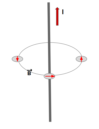
In 1820, Hans Oersted conducted a famous experiment using a compass needle and a current-carrying conductor. He observed that when no current was flowing through the conductor placed near the compass, the latter would always point towards the north pole. However, when the conductor was carrying a current, the needle deflected in a particular direction.
He found that the direction of deflection was tangent to a circle, which suggested that current-carrying wires produce a magnetic field around them (Figure 1). This magnetic field due to a urrent-carrying conductor can be calculated using the Biot-Savart law.
To estimate the magnetic field due to a current element, one can first calculate the differential field \(d\overrightarrow B \) and then integrate it over the loop. However, if we have a symmetry in the system, our calculations can be simplified using Ampere’s law.
Who Was André-Marie Ampere?
André-Marie Ampère, a French physicist and mathematician, displayed prodigious talents and began his study of mathematics at the early age of 12. His interest in the field of electromagnetism was sparked by Oersted’s discovery that electric currents produce magnetic fields.
Ampère expanded on Oersted’s work and demonstrated that current-carrying wires either repel or attract one another, depending on whether they were carrying current in the same or in opposite directions. One of his most significant contributions to the field is known as “Ampere’s Law” and in honor of his work, the SI unit of electric current is named after him.
Statement of Ampere’s Circuital law
Ampere’s law can be stated as follows: “The line integral of the magnetic field around any closed loop is proportional to the current passing through the loop.” If there are multiple currents passing through the loop, the algebraic sum of these currents must be taken into account and the loop considered for the calculation is called an “Amperian loop” or “Amperian coil.”
Note that the choice of the loop is aribtary and depends upon our ease of calculation.
Mathematical Form of Ampere’s Circuital Law
If we are given that a current is flowing through a given loop C, th
\[\oint {\vec B} \cdot \overrightarrow {dl} = {\mu _0}{i_{enc}}\]
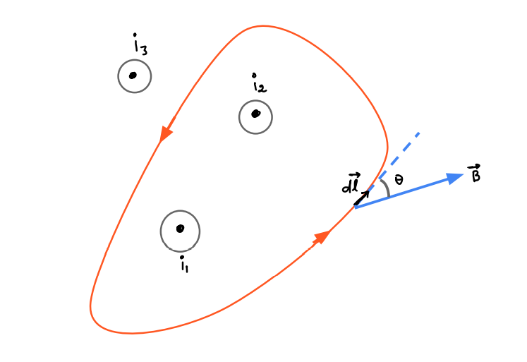
Line Integral of \(\overrightarrow B \) – The entire current loop can be divided into infinitesimally small subelements \(d\overrightarrow l \) . To calculate the total contribution, we simply integrate the tangential component of \(\overrightarrow B \) across the length of the loop.
Net current \({i_{enc}}\) – This is the current that is enclosed by the loop. Note that only those currents need to be taken into account which are inside the area of the loop.
From figure \({i_{enc}} = {i_1} + {i_2}\) only
Ampere’s circuital law
Direction of Integral – We can calculate the direction of the current and magnetic field using the right hand rule. If we curl our right hand such that our thumb points in the positive direction of current, our fingers will then point along the direction of magnetic field.
Inconsistency of Ampere’s Circuital Law
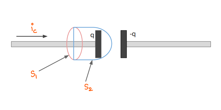
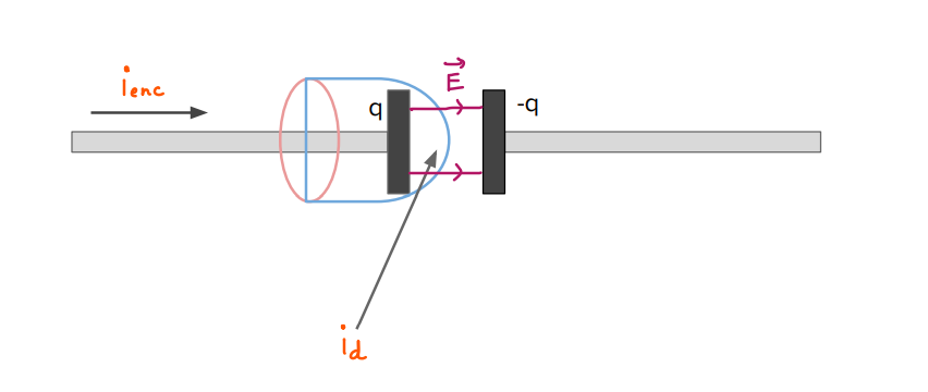
Take a look at the figure below and try to apply Ampere’s law to it. The circuit consists of a capacitor in a circuit wherein, a current \({i_c}\) is flowing.
Ampere’s circuital isn’t always valid.
Let us take two surfaces
- \({S_1}\): A simple circular loop wherein, \({i_{enc}}\) is simply \({i_{c}}\).
- The surface \({S_2}\)which is bulged out to the right. Since no current can flow in the gap of the capacitor, \({i_{enc}} = 0\).
Thus, we arrive at a discrepancy wherein, the line integral of magnetic field is both zero and non-zero.
Modified Ampere’s Circuital Law or Ampere – Maxwell’s Circuital Law
Maxwell modified Ampere’s law to remove the aforementioned discrepancy by introducing a term known as the displacement current. It is defined as:

Where E is the electric field passing through the loop. Notice how this term vanishes when the electric field is constant in time, leading us back to the original Ampere’s law. The modified form thus becomes
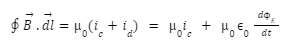
And the capacitor problem from before can now be solved:
Correction to Ampere’s law
This time, we notice that inside a capacitor, an electric field exists which varies in time and thus, the discrepancy has now been resolved.
Application of Ampere’s Circuital Law
There are a plethora of situations wherein, Ampere’s law comes in handy. As the first take example, let us calculate magnetic field due to a long wire at a distance r (r >> R)
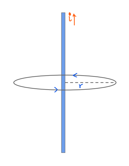
The magnetic field due to current-carrying wire.
The wire has cylindrical symmetry and we create a circular Amperian loop. Using the right hand rule, the direction of magnetic field comes out to be tangential to every point on the loop and thus,
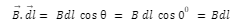
Ampere’s Law then states that
$$
\begin{gathered}
\oint \vec{B} \cdot \overrightarrow{d l}=\oint B d l=B \oint d l=B \cdot 2 \pi r=\mu_0 I \\
B=\frac{\mu_0{ }^i}{2 \pi r}
\end{gathered}
$$
This well-known result can also be verified via Biot-Savart law.
Solved Examples
Example 1. $$
\text { Find the value for } \vec{B} \cdot \overrightarrow{d l} \text { in surface } 1 \text { and } 2 \text { in units of } \mu_{0^{\circ}}
$$
Ans: Loop S1 contains two currents of values 1A and 5A. Thus,
$$
\vec{B} \cdot \overrightarrow{d l}=6
$$
Similarly, S2 has two currents, but one of them is in the negative direction. Therefore,
$$
\vec{B} \cdot \overrightarrow{d l}=5-2=3
$$
Example 2: A long straight wire of 2cm radius carries a current of 10A. Find the magnetic field at a distance of 8cm from it.
Ans: Using the equation previously derived,
$$
B=\frac{\mu_0{ }^2}{2 \pi r}=\frac{4 \Pi \times 10^7 \times 10}{2 \pi \times 8 \times 10^{-2}}=\frac{20 \times 10^{-3}}{8}=2.5 \times 10^{-5} \text { Tesla }
$$
Summary
Ampere’s law is a useful tool for estimating the magnetic field due to current distributions when the system exhibits some degree of symmetry. When time varying electric fields are present inside the loop, Ampere’s law fails to produce reasonable results. To address this limitation, Maxwell introduced the concept of Displacement current and a simple demonstration can be made using a capacitor.
Ampere’s law is particularly useful in estimating the magnetic field due to linear current carrying wires, where the magnitude of the field is inversely proportional to the distance at which it is being calculated.
Frequently Asked Questions
1. Apart from current carrying wires, what other sources can produce magnetic fields?
Time varying electric fields can produce magnetic fields.
2. Is ampere’s law universally true?
No. The law fails for dynamic cases and is only valid when no time-dependence exists.
3. Is it possible to derive Biot-Savart law from Ampere’s law?
Ampere’s law itself was derived using Biot-Savart law and thus, it is possible to interchange between the two.
4. For the case of electrostatics, is there a law equivalent to Ampere’s law?
Yes, Gauss’ law is almost congruent to Ampere’s law in electrostatics.
5. Summarize Ampere-Maxwell’s law?
Ampere Maxwell’s law proves how a changing electric field can produce a magnetic field, just as a changing magnetic field can induce an electric field (Faraday’s law).
 Mission Statement
“Empower every student to achieve full potential”
88Guru has been established with the social objective of making quality video-based learning material available to all Indian students. Technology, Connectivity and Social Media are rapidly changing the world of Education and we wish to lead the transformation of the tuition industry in India.
88Guru is the perfect complement to the current tuition model. 88Guru creates a wonderful opportunity for children and parents to bond while engaging in a valuable learning activity. It also provides the complete curriculum at your fingertips for those moments when you need some help at short notice. We believe that this mode of tuition could be transformational, adding hours to a child's day while providing complete control over the learning process.
Every course is taught by the best teachers from India's top schools and conducted in an engaging manner to keep students involved. The e-learning process consists of video-based instructions, computer-graded assignments, and a dashboard which allows the student and parent to track progress.